Machine Learning Paradigms: Advances in Data Analytics — A Complete Engineering Guide
Introduction
Machine learning (ML) has transformed data analytics from a largely descriptive discipline into a predictive and increasingly autonomous engineering capability. Instead of simply asking “What happened?”, modern analytics systems can ask “What is likely to happen?”, “Why is it happening?”, and even “What action should be taken next?” 🤖📊
For engineering students and professionals, understanding machine learning paradigms is particularly important because engineering systems continuously generate data. Sensors, industrial controllers, production lines, energy meters, vehicles, satellites, medical instruments, and software platforms can produce millions of observations every day.
The major machine learning paradigms—including supervised learning, unsupervised learning, semi-supervised learning, self-supervised learning, reinforcement learning, and hybrid approaches—provide different strategies for extracting knowledge from these datasets.
The evolution is significant. Traditional analytics often depended on predefined rules and manually designed statistical models. Modern ML systems can discover complex relationships, identify anomalies, classify objects, forecast failures, optimize processes, and support engineering decisions.


This article explains the theory, definitions, workflows, comparisons, engineering applications, practical examples, challenges, and future direction of machine learning paradigms in data analytics.
Background Theory
From Traditional Analytics to Machine Learning
Traditional data analytics generally follows a structured sequence:
Data → Cleaning → Statistical Analysis → Visualization → Decision
For example, an engineer analyzing a manufacturing plant might calculate the average temperature of a machine and compare it with historical limits.
Machine learning introduces a different approach:
Data → Features/Representation → Learning Algorithm → Model → Prediction/Decision
Instead of manually specifying every relationship, an algorithm learns patterns from historical observations.
A simplified learning problem can be expressed as:
[f:X\rightarrow Y]
where:
- (X) = input data
- (Y) = desired output
- (f) = learned function
For regression, the model may estimate:
[\hat{y}=f(x)]
For classification, it may estimate the probability of a class:
[P(y=k|x)]
The quality of the resulting model depends on data quality, feature representation, algorithm selection, training methodology, and evaluation.
Why Paradigms Matter
A machine learning paradigm determines how a model learns.
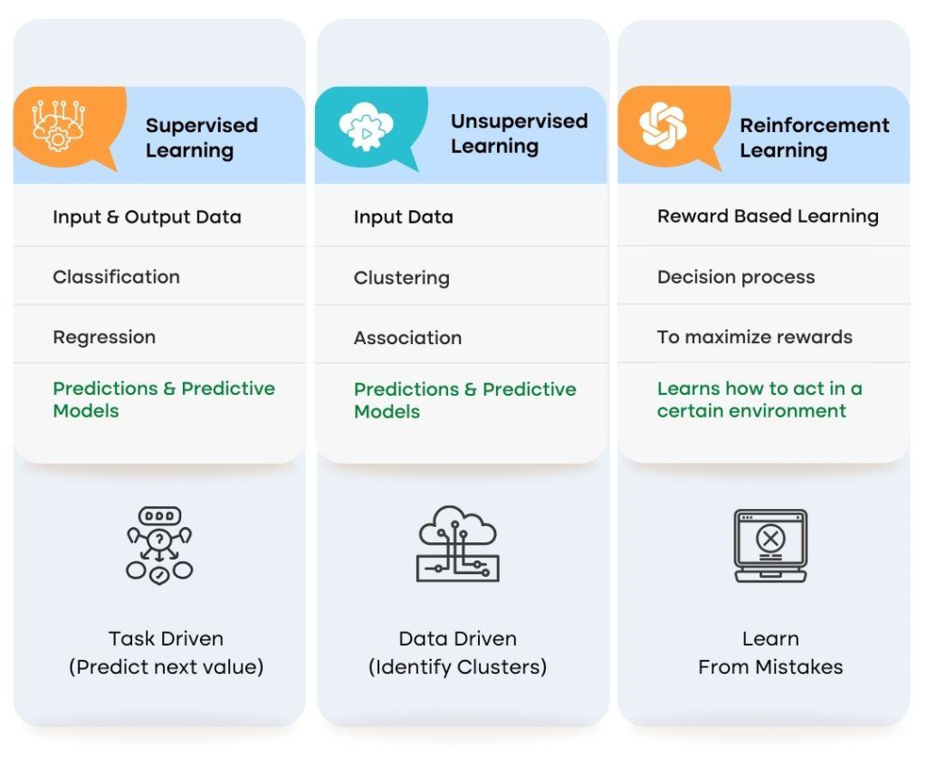
📊 If historical data contains known answers, supervised learning may be appropriate. If there are no labels, unsupervised learning can reveal hidden structures. If an agent must repeatedly interact with an environment and learn from rewards, reinforcement learning becomes more appropriate.
Therefore, choosing the correct paradigm is an engineering decision—not merely a programming decision. ⚙️
Definition
What Is a Machine Learning Paradigm?
A machine learning paradigm is a fundamental approach describing how an algorithm learns patterns, relationships, representations, or decisions from data and interaction with an environment.
The major paradigms include:
| Paradigm | Main Learning Signal | Typical Objective |
|---|---|---|
| Supervised Learning | Labeled examples | Prediction |
| Unsupervised Learning | Data structure | Pattern discovery |
| Semi-Supervised Learning | Few labels + many unlabeled samples | Improved prediction |
| Self-Supervised Learning | Automatically generated targets | Representation learning |
| Reinforcement Learning | Rewards and penalties | Sequential decision-making |
| Hybrid Learning | Multiple learning strategies | Complex engineering problems |
The choice depends on the available data and the engineering objective.
Supervised Learning
In supervised learning, the algorithm receives input-output examples:
[D={(x_i,y_i)}_{i=1}^{n}]
The objective is to learn a function that maps inputs to appropriate outputs.
Common applications include:
- Failure prediction
- Demand forecasting
- Image classification
- Quality inspection
- Energy consumption prediction
- Equipment remaining-useful-life estimation
Typical algorithms include linear regression, logistic regression, decision trees, random forests, support vector machines, and neural networks.
Unsupervised Learning
Unsupervised learning operates without predefined output labels.
Given:
[D={x_1,x_2,\ldots,x_n}]
the algorithm attempts to discover structures within the dataset.
Examples include:
- Customer segmentation
- Sensor anomaly detection
- Equipment clustering
- Dimensionality reduction
- Pattern discovery
Popular techniques include K-means clustering, hierarchical clustering, DBSCAN, PCA, and autoencoders.
Semi-Supervised Learning
Engineering datasets frequently contain thousands or millions of measurements but only a small number of professionally labeled observations.
Semi-supervised learning combines:
[D_L=\text{labeled data}]
with:
[D_U=\text{unlabeled data}]
This can be valuable when labeling requires expensive laboratory testing or expert inspection.
Self-Supervised Learning
Self-supervised learning creates learning targets from the data itself.
For example, a model could receive part of a signal and attempt to predict the missing section.
This approach has become increasingly important for large-scale representation learning because massive quantities of unlabeled data can be utilized.
Reinforcement Learning
Reinforcement learning is fundamentally different.
An agent interacts with an environment:
[State \rightarrow Action \rightarrow Reward \rightarrow New\ State]
The objective is to maximize cumulative reward:
[G_t=\sum_{k=0}^{\infty}\gamma^kR_{t+k+1}]
where:
- (R) = reward
- (\gamma) = discount factor
- (G_t) = return
Engineering applications include robotics, autonomous systems, process optimization, energy management, and traffic control.
Step-by-Step Explanation
Step 1: Define the Engineering Problem
Start with the physical or business problem—not the algorithm.
For example:
Can machine vibration measurements be used to predict bearing failure?
This establishes the target variable and operational objective.
Step 2: Collect Data
Potential sources include:
- IoT sensors
- SCADA systems
- Laboratory experiments
- Maintenance records
- Manufacturing databases
- Simulation software
- Images and video
- Historical operational logs
Data may contain:
[X=[temperature,\ vibration,\ pressure,\ speed,\ load]]
Step 3: Clean the Dataset
Real engineering data is rarely perfect.
Common problems include missing measurements, sensor drift, duplicate observations, inconsistent units, and extreme outliers.
A basic preprocessing workflow is:
Raw Data → Validation → Cleaning → Transformation → Dataset
Step 4: Select the Learning Paradigm
Ask:
Do I have labels?
- Yes → supervised learning
- No → unsupervised learning
- Few labels → semi-supervised learning
- Huge unlabeled dataset → self-supervised learning
- Sequential decisions → reinforcement learning
Step 5: Engineer or Learn Representations
For conventional ML, engineers may calculate:
[RMS=\sqrt{\frac{1}{N}\sum_{i=1}^{N}x_i^2}]
for vibration signals.
Other features may include:
- Mean
- Standard deviation
- Peak amplitude
- Frequency components
- Kurtosis
- Skewness
- Temperature gradient
Deep learning models can instead learn representations directly from raw data.
Step 6: Train the Model
The dataset is normally divided into:
- Training set
- Validation set
- Test set
The model minimizes an objective such as mean squared error:
[MSE=\frac{1}{n}\sum_{i=1}^{n}(y_i-\hat{y_i})^2]
Step 7: Evaluate Performance
Different problems require different metrics.
For classification:
[Accuracy=\frac{TP+TN}{TP+TN+FP+FN}]
Other important metrics include precision, recall, F1-score, ROC-AUC, and confusion matrices.
For regression, engineers may use MAE, MSE, RMSE, and (R^2).
Step 8: Deploy and Monitor
Deployment is not the final step.
Real systems must continuously monitor:
Prediction Quality → Data Drift → Model Drift → Retraining


Comparison
Machine Learning Paradigms Compared
| Characteristic | Supervised | Unsupervised | Semi-Supervised | Self-Supervised | Reinforcement |
|---|---|---|---|---|---|
| Labels | Required | No | Limited | Automatically generated | Rewards |
| Main Goal | Prediction | Discovery | Prediction | Representation | Decision |
| Human Labeling | High | Low | Moderate | Low | Environment dependent |
| Typical Output | Class/value | Clusters/features | Class/value | Learned representation | Action |
| Engineering Example | Failure prediction | Fault clustering | Defect detection | Sensor representation | Robot control |
Traditional Analytics vs Machine Learning
Traditional analytics often relies on explicit mathematical assumptions and predefined relationships.
Machine learning is more flexible when relationships are nonlinear or difficult to model manually.
However, ML is not automatically superior.
For a simple engineering relationship such as:
[
F=ma
]
a physics-based model is generally more interpretable and reliable than training a neural network to rediscover the same relationship.
The strongest modern systems often combine physics, statistics, and machine learning. 🧠⚙️
Diagrams & Tables
A General ML Data Analytics Architecture
              ┌──────────────────┐
              │ Engineering Data │
              └────────┬─────────┘
                       ↓
              ┌──────────────────┐
              │ Data Preparation │
              └────────┬─────────┘
                       ↓
              ┌──────────────────┐
              │ Learning         │
              │ Paradigm         │
              └────────┬─────────┘
                       ↓
              ┌──────────────────┐
              │ ML Model         │
              └────────┬─────────┘
                       ↓
              ┌──────────────────┐
              │ Prediction /     │
              │ Decision         │
              └────────┬─────────┘
                       ↓
              ┌──────────────────┐
              │ Monitoring       │
              └──────────────────┘


Selecting a Paradigm
| Engineering Question | Recommended Approach |
|---|---|
| Will this component fail? | Supervised learning |
| Which machines behave similarly? | Unsupervised learning |
| Only some failures are labeled? | Semi-supervised learning |
| Massive unlabeled sensor dataset? | Self-supervised learning |
| Which control action is optimal? | Reinforcement learning |
| Strong physical laws plus data? | Hybrid/physics-informed ML |
Examples
Example 1: Predictive Maintenance
Suppose an industrial motor produces vibration measurements every second.
The dataset contains:
[X=[vibration, temperature, current, speed, load]]
and maintenance records identify whether a failure occurred.
A supervised model can learn:
[P(Failure|X)]
If the probability exceeds an engineering threshold, maintenance can be scheduled.
The advantage is substantial: maintenance can potentially move from reactive to predictive.
Example 2: Manufacturing Quality
A production line produces thousands of components.
A camera captures each component, while inspection engineers label defective products.
A computer vision model can learn the relationship:
[Image \rightarrow Defect/Accept]
This can automate repetitive inspection and provide consistent screening.
Example 3: Energy Forecasting
A building may contain historical electricity measurements along with:
- Outdoor temperature
- Humidity
- Occupancy
- Day of week
- Time
- Equipment operating state
A regression model can estimate future energy demand.
This supports:
[Demand\ Forecasting \rightarrow Load\ Planning \rightarrow Energy\ Optimization]
Real World Application
Industrial Engineering
Machine learning can analyze equipment signals to identify abnormal behavior before catastrophic failure occurs.
Civil Engineering
ML can support:
- Structural health monitoring
- Traffic prediction
- Construction progress analysis
- Concrete strength prediction
- Infrastructure defect detection
Mechanical Engineering
Applications include:
- Predictive maintenance
- Fault diagnosis
- Design optimization
- Computational simulation acceleration
- Robotics
Electrical Engineering
ML is increasingly useful for:
- Load forecasting
- Renewable energy prediction
- Power-quality analysis
- Fault detection
- Grid optimization
Aerospace Engineering
Aircraft and spacecraft generate enormous quantities of sensor data.
ML can assist with:
- Anomaly detection
- Predictive maintenance
- Flight-data analysis
- Trajectory optimization
- Component health monitoring
Software and Data Engineering
Modern software systems use ML for:
- Log anomaly detection
- Performance forecasting
- Recommendation systems
- Fraud detection
- Automated classification
Common Mistakes
Choosing the Algorithm Before Understanding the Problem
A common mistake is starting with:
“Which neural network should I use?”
The better question is:
“What information is available, what is the objective, and what type of learning signal exists?”
Ignoring Data Leakage
Data leakage occurs when information unavailable at prediction time enters the training process.
This can produce impressive test results but poor real-world performance.
Using Accuracy Alone
A model detecting rare failures could achieve 99% accuracy by predicting “no failure” almost every time.
For imbalanced engineering datasets, precision, recall, F1-score, and cost-sensitive metrics may be more informative.
Ignoring Physical Constraints
A model can generate mathematically plausible but physically impossible predictions.
Engineering ML should respect constraints such as:
[Mass>0]
[Temperature \geq 0\ K]
and conservation laws where applicable.
Treating Model Deployment as the End
A model trained today may degrade when operating conditions change.
Continuous monitoring is essential.
Challenges & Solutions
Poor Data Quality
Challenge: Missing, noisy, or inconsistent sensor measurements.
Solution: Establish data validation, calibration procedures, filtering, imputation, and quality-control pipelines.
Limited Labeled Data
Challenge: Expert labeling can be expensive.
Solution: Consider semi-supervised learning, active learning, transfer learning, or self-supervised learning.
Model Interpretability
Challenge: Complex models may be difficult to explain.
Solution: Use interpretable models when appropriate and apply explainability methods such as feature importance, sensitivity analysis, and local explanations.
Data Drift
Challenge: Operating conditions change over time.
Solution: Monitor statistical distributions and model performance and establish retraining criteria.
Computational Cost
Challenge: Large deep learning models may require substantial computing resources.
Solution: Use model compression, efficient architectures, feature selection, or simpler models when they provide adequate performance.
Case Study
Predictive Maintenance for an Industrial Pump
Consider an industrial pumping system operating continuously.
Sensors measure:
- Vibration
- Pressure
- Temperature
- Flow rate
- Motor current
- Rotational speed
Initially, engineers use fixed thresholds:
[Vibration>V_{limit}]
When the threshold is exceeded, maintenance is triggered.
However, this approach can produce false alarms because vibration may increase temporarily during certain operating conditions.
An ML-based system can learn relationships among multiple variables.
For example:
[Failure=f(V,T,P,Q,I,S)]
where:
- (V) = vibration
- (T) = temperature
- (P) = pressure
- (Q) = flow
- (I) = current
- (S) = speed
The system can distinguish between normal high vibration during a particular operating state and vibration patterns associated with actual deterioration.
A practical implementation could involve:
Sensors → Data Historian → Feature Engineering → ML Model → Failure Probability → Maintenance Decision
The key engineering benefit is not simply higher prediction accuracy. It is the ability to connect predictions to maintenance planning, inventory management, downtime reduction, and operational safety.
Essential Tips
Start With Engineering Knowledge
Machine learning should complement engineering expertise rather than replace it.
Build a Strong Data Pipeline
A sophisticated algorithm cannot compensate for unreliable measurements.
Establish a Baseline
Always compare ML against:
- Existing engineering rules
- Statistical models
- Simple regression
- Historical averages
A complex model should demonstrate measurable value.
Validate With Real Operating Conditions
Random train-test splits may be inappropriate for time-dependent engineering data.
For temporal datasets, chronological validation is often more realistic:
[Past\ Data \rightarrow Training]
[Future\ Data \rightarrow Testing]
Monitor the Model
Track:
[Accuracy,\ Drift,\ Latency,\ Reliability,\ Cost]
rather than accuracy alone.
Combine Physics and Data
Where physical laws are known, use them.
The future of engineering ML is unlikely to be purely data-driven. Hybrid systems combining physics-based modeling + machine learning + domain knowledge can be especially powerful. 🔬⚙️
FAQs
What are the main machine learning paradigms?
The major paradigms are supervised, unsupervised, semi-supervised, self-supervised, and reinforcement learning. Hybrid approaches can combine multiple paradigms.
Which paradigm is best for engineering?
There is no universal best paradigm. Supervised learning is useful when labeled historical data exists, while unsupervised learning is useful for discovering patterns. Reinforcement learning is better suited to sequential decision and control problems.
Is machine learning replacing traditional engineering models?
Not necessarily. Engineering models based on physics remain extremely valuable. Machine learning often complements them by modeling complex relationships, estimating unknown parameters, detecting anomalies, or accelerating computational workflows.
Why is data quality important in machine learning?
ML models learn from data. Incorrect, biased, incomplete, or poorly measured data can produce unreliable predictions regardless of how advanced the algorithm is.
Can machine learning work without labeled data?
Yes. Unsupervised and self-supervised approaches can learn from unlabeled datasets, while semi-supervised learning can combine a small labeled dataset with a much larger unlabeled dataset.
What is the difference between machine learning and data analytics?
Data analytics traditionally focuses on extracting insights from data through statistics, visualization, and analysis. Machine learning adds algorithms capable of learning patterns for prediction, classification, representation, or decision-making.
Why is explainability important in engineering?
Engineering decisions can affect safety, cost, reliability, and regulatory compliance. Engineers therefore often need to understand why a model produced a particular result rather than relying solely on a numerical prediction.
What is the future of machine learning in engineering?
Future systems are likely to combine machine learning with physics-based simulation, digital twins, edge computing, IoT, autonomous systems, generative AI, and advanced optimization techniques.
Conclusion
Machine learning paradigms have fundamentally expanded the capabilities of modern data analytics. Instead of treating data merely as historical records, engineers can use it as a source of prediction, optimization, anomaly detection, automated decision-making, and system intelligence. 🚀
Supervised learning provides powerful predictive capabilities when labeled data is available. Unsupervised learning discovers hidden structures. Semi-supervised and self-supervised approaches address the practical problem of limited labeling. Reinforcement learning introduces learning through interaction and rewards.
For engineering applications, however, selecting an algorithm is only one part of the solution. Successful ML systems require reliable sensors, carefully prepared datasets, appropriate validation, meaningful performance metrics, domain expertise, and continuous monitoring.
The most promising direction is therefore not simply “more artificial intelligence.” It is the integration of machine learning + engineering principles + statistical reasoning + physical models + high-quality data.
As engineering systems become increasingly connected and data-rich, professionals who understand these paradigms will be better prepared to transform raw measurements into actionable intelligence—and ultimately build systems that are more predictive, efficient, reliable, and autonomous. ⚙️📊🤖