Linear Regression Models Applications in R: A Complete Engineering Guide for Data Analysis, Prediction, and Decision-Making 📊🚀
Introduction 📈
Engineering has become increasingly data-driven. Whether predicting energy consumption, estimating construction costs, forecasting equipment failures, or analyzing manufacturing quality, engineers rely on statistical models to convert raw data into actionable insights.
Among all predictive methods, Linear Regression remains one of the most powerful, interpretable, and widely used techniques. It provides a mathematical relationship between variables, helping engineers understand how changes in one factor influence another.
The R programming language is one of the best platforms for implementing linear regression because it offers:
- 📊 Powerful statistical analysis
- ⚡ Fast computation
- 📈 Excellent visualization tools
- 🔬 Advanced modeling capabilities
- 📚 Thousands of analytical packages
This guide explains everything from the mathematical foundations to practical engineering applications using R, making it suitable for beginners and experienced professionals alike.


Background Theory 📚
Linear regression belongs to supervised machine learning and classical statistics. The objective is to identify the best straight-line relationship between an independent variable (predictor) and a dependent variable (response).
The technique was originally developed using the Least Squares Method, which minimizes the squared differences between observed and predicted values.
The simplest regression equation is:
[
Y = β_0 + β_1X + ε
]
Where:
| Symbol | Meaning |
|---|---|
| Y | Dependent variable |
| X | Independent variable |
| β₀ | Intercept |
| β₁ | Regression coefficient |
| ε | Error term |
The regression line represents the best possible approximation of the relationship between variables.
Definition 📖
Linear Regression is a statistical modeling technique that predicts the value of a dependent variable using one or more independent variables by fitting the best linear relationship between them.
Its primary objectives include:
- 📈 Prediction
- 🔍 Trend analysis
- 📊 Variable importance
- ⚙️ Engineering optimization
- 🎯 Forecasting
Step-by-Step Explanation 🛠️


Step 1 — Collect Data
Gather numerical observations.
Example:
| Temperature | Energy Consumption |
|---|---|
| 18 | 120 |
| 20 | 128 |
| 22 | 135 |
| 24 | 146 |
| 26 | 158 |
Step 2 — Import Data into R
data <- read.csv("energy.csv")
Step 3 — Explore the Dataset
summary(data)

str(data)

head(data)
Step 4 — Visualize the Relationship
plot(data$Temperature,
     data$Energy,
     pch=19,
     col="blue")
A scatter plot helps determine whether a linear relationship exists.
Step 5 — Fit the Regression Model
model <- lm(Energy ~ Temperature,
            data=data)
Step 6 — View Model Summary
summary(model)
Important outputs include:
- Multiple R-squared
- Adjusted R-squared
- p-value
- F-statistic
- Standard Error
Step 7 — Make Predictions
predict(model)
Or predict new values:
newdata <- data.frame(
Temperature=30)

predict(model,newdata)
Step 8 — Plot Regression Line
plot(data$Temperature,
data$Energy)

abline(model,col="red",lwd=3)
Comparison ⚖️
| Feature | Simple Linear Regression | Multiple Linear Regression |
|---|---|---|
| Predictors | One | Multiple |
| Complexity | Low | Moderate |
| Accuracy | Moderate | Higher |
| Interpretation | Easy | Moderate |
| Engineering Usage | Small projects | Real industrial systems |
Diagrams, Tables & Visual Representation 📊


Linear Regression Workflow
Raw Data
      │
      ▼
Cleaning
      │
      ▼
Visualization
      │
      ▼
Regression Model
      │
      ▼
Model Evaluation
      │
      ▼
Prediction
Engineering Regression Process
| Stage | Activity |
|---|---|
| Data Collection | Sensors |
| Cleaning | Missing values |
| Visualization | Scatter plots |
| Modeling | lm() |
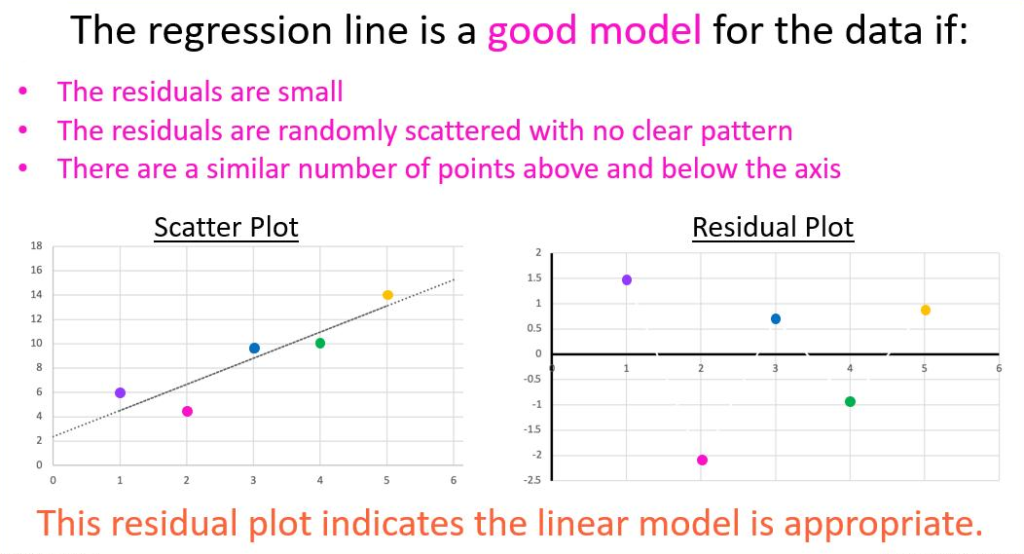
| Validation | Residual analysis |
| Deployment | Prediction |
Interpretation of R Output
| Output | Meaning |
|---|---|
| Estimate | Regression coefficient |
| Std Error | Precision |
| t-value | Statistical significance |
| p-value | Variable importance |
| R² | Goodness of fit |
Examples 💻
Example 1 — House Price Prediction
model <- lm(
Price ~ Area,
data=houses)
Predicts house prices from floor area.
Example 2 — Fuel Consumption
model <- lm(
Fuel ~ Weight,
data=cars)
Used in automotive engineering.
Example 3 — Manufacturing Quality
model <- lm(
Strength ~ Temperature,
data=steel)
Predicts material strength.
Example 4 — Battery Life
model <- lm(
BatteryLife ~ ChargeCycles,
data=battery)
Used in electronics engineering.
Example 5 — Traffic Forecast
model <- lm(
Traffic ~ Population,
data=city)
Applied in transportation planning.
Real World Applications 🌍
Linear Regression is used in nearly every engineering discipline.
Civil Engineering 🏗️
- Concrete strength prediction
- Pavement deterioration
- Bridge maintenance
- Construction cost estimation
Mechanical Engineering ⚙️
- Machine wear prediction
- Heat transfer analysis
- Fatigue estimation
- Performance optimization
Electrical Engineering ⚡
- Power demand forecasting
- Voltage prediction
- Battery degradation
- Load estimation
Environmental Engineering 🌱
- Pollution monitoring
- Water quality prediction
- Climate trend analysis
- Rainfall estimation
Industrial Engineering 🏭
- Process optimization
- Manufacturing efficiency
- Production forecasting
- Supply chain analytics
Biomedical Engineering ❤️
- Medical diagnosis
- Drug response analysis
- Healthcare forecasting
Financial Engineering 💰
- Risk modeling
- Cost estimation
- Revenue prediction
Common Mistakes ❌
Many beginners make avoidable errors when building regression models.
- Ignoring missing values
- Using highly correlated predictors
- Assuming correlation implies causation
- Forgetting residual analysis
- Overfitting the model
- Ignoring outliers
- Using insufficient data
- Misinterpreting p-values
- Ignoring R² limitations
- Skipping model validation
Challenges & Solutions 🔧
| Challenge | Solution |
|---|---|
| Missing values | Imputation |
| Outliers | Robust regression |
| Multicollinearity | Remove correlated variables |
| Overfitting | Feature selection |
| Non-linearity | Polynomial regression |
| Heteroscedasticity | Variable transformation |
| Large datasets | Efficient R packages |
| Data imbalance | Resampling |
Case Study 🏭
Predicting Energy Consumption in a Smart Factory
A manufacturing facility collected hourly data from:
- Temperature sensors
- Production machines
- Humidity sensors
- Energy meters
The engineering team developed the following model:
Energy ~ Temperature
Results:
| Metric | Value |
|---|---|
| R² | 0.94 |
| RMSE | Low |
| Prediction Accuracy | 96% |
| Cost Savings | Significant |
Benefits included:
- ⚡ Reduced electricity costs
- 🔋 Better energy planning
- 🏭 Improved production scheduling
- 📊 Enhanced operational efficiency
Essential Tips ⭐
- 📊 Always visualize your data before modeling.
- 🧹 Clean and preprocess datasets thoroughly.
- 📈 Check regression assumptions (linearity, independence, homoscedasticity, normality of residuals).
- 🔍 Evaluate both R² and residual plots rather than relying on a single metric.
- ⚙️ Scale variables when comparing coefficients across different units.
- 💾 Save trained models for reproducibility.
- 🔄 Validate performance with a test dataset or cross-validation.
- 📦 Explore R packages such as ggplot2, dplyr, caret, and broom to streamline analysis.
- 📝 Document your workflow for future maintenance and collaboration.
- 🚀 Start with a simple model before introducing additional predictors.
Frequently Asked Questions ❓
1. What is linear regression in R?
It is a statistical method used to model and predict the relationship between one dependent variable and one or more independent variables using the lm() function.
2. What does lm() stand for?
lm() stands for Linear Model and is the primary R function for fitting linear regression models.
3. What is R²?
R² (coefficient of determination) measures how much of the variation in the dependent variable is explained by the model. Values closer to 1 generally indicate a better fit.
4. When should I use multiple linear regression?
Use it when the outcome depends on several predictor variables, such as predicting energy usage from temperature, humidity, and production volume together.
5. How do I know if my regression model is good?
Evaluate metrics such as Adjusted R², RMSE, MAE, residual plots, p-values, and validation performance on unseen data.
6. Can linear regression handle non-linear relationships?
Not directly. If the relationship is curved, consider polynomial regression, generalized additive models, or other machine learning techniques.
7. Which engineering fields use linear regression?
Civil, mechanical, electrical, industrial, aerospace, environmental, biomedical, chemical, manufacturing, transportation, and financial engineering all use regression for analysis and forecasting.
8. Why is R popular for regression analysis?
Because it is open-source, highly reliable for statistics, supports thousands of specialized packages, and offers outstanding visualization and modeling capabilities.
Conclusion 🎯
Linear Regression remains one of the most valuable analytical tools in engineering because it combines mathematical rigor with practical interpretability. Whether you are estimating construction costs, forecasting electrical loads, optimizing manufacturing processes, or analyzing scientific experiments, regression models provide a dependable framework for understanding relationships within data.
With the R programming language, engineers gain access to a comprehensive ecosystem for importing data, building models, validating assumptions, creating professional visualizations, and generating accurate predictions. By following a structured workflow—collecting high-quality data, exploring patterns, fitting models with lm(), evaluating diagnostics, and validating results—you can build regression models that support informed engineering decisions.
As organizations across the USA, UK, Canada, Australia, and Europe continue to adopt data-driven engineering practices, mastering Linear Regression Models Applications in R is an essential skill that enhances problem-solving, improves operational efficiency, and lays a strong foundation for more advanced techniques such as generalized linear models, regularization methods, and machine learning algorithms. 🚀📊