Bayesian Data Analysis 2nd Edition: A Complete Engineering Guide to Bayesian Statistics, Modeling, and Decision-Making 📊🔬🚀
Introduction 🌟
In the modern era of engineering, artificial intelligence, data science, reliability analysis, and predictive modeling, uncertainty is everywhere. Engineers constantly make decisions based on incomplete information, noisy measurements, and changing environments. Traditional statistical approaches often struggle when dealing with limited data or evolving knowledge.
This is where Bayesian Data Analysis 2nd Edition becomes one of the most influential references in modern statistical science. Written by renowned statisticians Andrew Gelman, John B. Carlin, Hal S. Stern, and Donald B. Rubin, the book provides a practical and theoretical framework for understanding uncertainty through Bayesian methods.
Unlike classical statistics, which treats parameters as fixed but unknown values, Bayesian statistics allows engineers and researchers to continuously update beliefs as new information becomes available. This creates a dynamic decision-making process that closely matches how real-world engineering systems operate.
Whether you are an engineering student learning probability theory or a professional working with machine learning models, reliability systems, financial forecasting, or industrial optimization, Bayesian Data Analysis offers powerful tools for extracting knowledge from data.
📈 Bayesian thinking is now widely used in:
- Artificial Intelligence
- Machine Learning
- Signal Processing
- Robotics
- Manufacturing
- Aerospace Engineering
- Medical Engineering
- Quality Control
- Risk Assessment
- Financial Engineering
This guide explores the major concepts, theories, methodologies, and practical applications associated with Bayesian Data Analysis 2nd Edition.
Background Theory 🧠
Origins of Bayesian Statistics
Bayesian statistics originates from the work of the English mathematician:
Thomas Bayes
Bayes developed a theorem describing how probabilities can be updated when new evidence becomes available.
The Bayesian framework remained relatively obscure for many years because calculations were computationally difficult.
The rise of modern computers in the late twentieth century transformed Bayesian statistics into one of the most powerful analytical methodologies available today.
Fundamental Philosophy
The Bayesian approach treats probability as a measure of belief rather than merely a frequency of occurrence.
Suppose an engineer believes there is a 60% chance that a machine component will fail within one year.
After collecting additional sensor data, that belief may increase to 80% or decrease to 30%.
Bayesian analysis provides the mathematical mechanism for updating those beliefs.
This process mimics human reasoning:
🌟 Prior Knowledge
➡️ New Evidence
➡️ Updated Understanding
Bayes’ Theorem
The foundation of Bayesian analysis is:
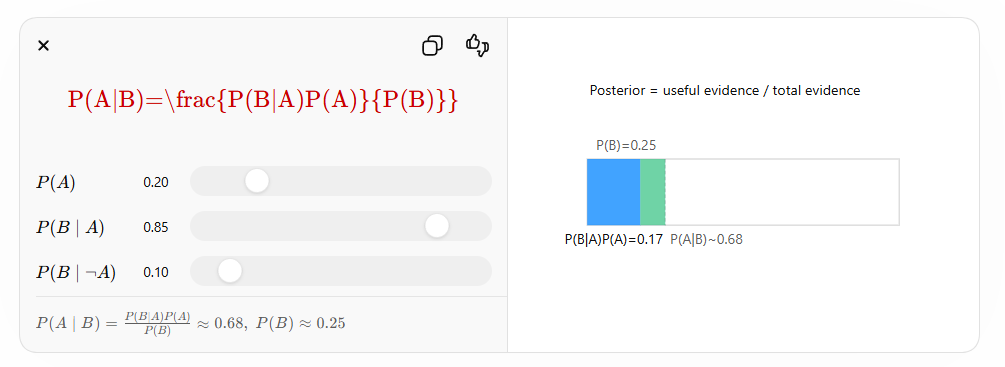
Where:
- P(A) = Prior Probability
- P(B|A) = Likelihood
- P(B) = Evidence
- P(A|B) = Posterior Probability
The posterior probability becomes the updated belief after observing data.
Technical Definition ⚙️
Bayesian Data Analysis is a statistical methodology that combines:
- Prior information
- Observed data
- Probability models
to estimate unknown parameters and make predictions.
Mathematically:
Posterior ∝ Prior × Likelihood
The goal is not merely to estimate a single value but to describe the entire probability distribution of possible outcomes.
Key components include:
Prior Distribution
Represents knowledge before observing data.
Examples:
- Historical measurements
- Expert opinions
- Previous experiments
Likelihood Function
Describes how likely the observed data are under different parameter values.
Posterior Distribution
Represents updated knowledge after incorporating observations.
Predictive Distribution
Forecasts future outcomes using the posterior distribution.
Core Concepts in Bayesian Data Analysis 🔍
Prior Probability
Prior distributions can be:
Informative Priors
Built from existing knowledge.
Examples:
- Previous reliability studies
- Historical production data
Non-Informative Priors
Used when little prior knowledge exists.
Examples:
- Uniform distributions
- Weakly informative assumptions
Posterior Probability
The posterior combines data and prior information.
Benefits include:
🌟 Better estimates with small datasets
✅ Incorporation of expert knowledge
✅ Explicit uncertainty quantification
Hierarchical Models
One of the major strengths of Bayesian Data Analysis 2nd Edition is its extensive discussion of hierarchical models.
These models handle data with multiple levels.
Examples:
- Schools within districts
- Machines within factories
- Sensors within networks
Hierarchical structures improve prediction accuracy and reduce overfitting.
Markov Chain Monte Carlo (MCMC)
Many Bayesian problems cannot be solved analytically.
MCMC algorithms generate samples from posterior distributions.
Popular methods include:
- Gibbs Sampling
- Metropolis-Hastings
- Hamiltonian Monte Carlo
These techniques transformed Bayesian analysis into a practical engineering tool.
Step-by-Step Bayesian Analysis Process 🚀
Step 1: Define the Problem
Example:
Estimate the failure rate of a hydraulic pump.
Questions include:
- What parameter is unknown?
- What data are available?
Step 2: Specify a Prior
Historical records suggest:
Failure probability ≈ 5%
This becomes the prior distribution.
Step 3: Collect Data
Suppose:
- 100 pumps tested
- 8 failures observed
Observed data become the evidence.
Step 4: Build the Likelihood
Model the failures using:
- Binomial distribution
- Poisson distribution
- Normal distribution
depending on the problem.
Step 5: Calculate Posterior Distribution
Combine:
Prior × Likelihood
to obtain updated probabilities.
Step 6: Validate Results
Check:
✔ Convergence
✔ Residual analysis
🌟 Posterior predictive checks
✔ Sensitivity analysis
Step 7: Make Decisions
Examples:
- Replace equipment
- Schedule maintenance
- Adjust manufacturing parameters
Comparison: Bayesian vs Frequentist Statistics ⚖️
| Feature | Bayesian Statistics | Frequentist Statistics |
|---|---|---|
| Prior Knowledge | Included | Ignored |
| Interpretation | Probability of belief | Long-run frequency |
| Output | Probability distributions | Point estimates |
| Small Data Performance | Strong | Often weaker |
| Updating Results | Easy | Difficult |
| Uncertainty Representation | Excellent | Limited |
| Computational Cost | Higher | Lower |
Engineering Perspective
Bayesian methods are often preferred when:
- Data are limited
- Expert knowledge exists
- Risk estimation is critical
Frequentist methods remain useful when:
- Large datasets exist
- Fast computation is required